Big Data on AWS Deep Dive (Part 7): Recommendation System Fundamentals — Funnel, Two-Tower, and PIT

Once data lands in the lake, the ultimate goal is to serve recommendation algorithms. This chapter covers recommendation systems from scratch: the recall-ranking funnel, feature engineering, model types, and why PIT correctness is the critical lifeline.

No ML background assumed — just familiarity with code and basic concepts like “vector” and “dot product.”

---

What Problem Does a Recommendation System Solve?#

When you scroll through TikTok, Instagram, or YouTube, you see different content every time you open the app — there is a recommendation system working behind the scenes.

It must answer: “From hundreds of millions of candidates, which 10 items should this specific user see? Decide within 200ms.”

The challenges:

1. Too many candidates: Platforms receive tens of millions of new uploads daily with hundreds of millions of active users
2. Strict latency: User-perceived response must be under 200ms
3. Personalization at scale: Every user has different preferences
4. Real-time feedback: If a user taps “not interested,” the next refresh must reflect that
5. Cold start: New users have no history; new content has no engagement data

Scoring and ranking every candidate for every user is computationally impossible within latency budgets. That is why we need a multi-stage filtering “funnel.”

---

The Recommendation Funnel: 4–5 Stages#

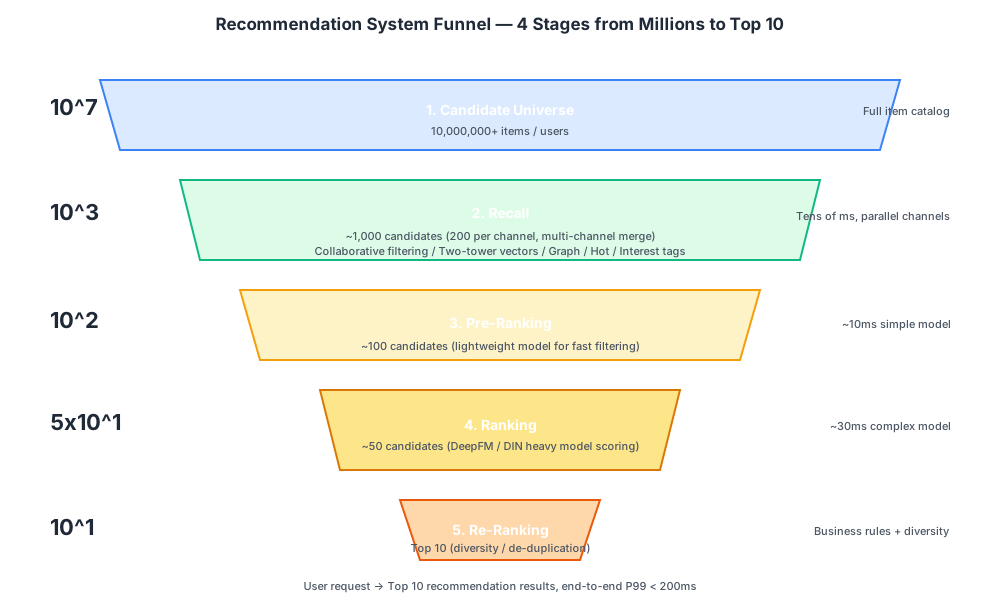
Stage 1: Candidate Pool (10^7 scale)#

The entire content library or user graph. This is the raw source data.

Stage 2: Recall (down to 10^3)#

Quickly filter hundreds of millions of candidates down to a few hundred or thousand for downstream models to score.

Multi-channel recall — run N different retrieval methods in parallel, then merge results:

Recall Channel	Method	Data Source
Collaborative Filtering (U2U-CF / I2I-CF)	“Users similar to you liked these”	Historical interaction matrix
Two-Tower vector recall	User vector → find nearest-neighbor item vectors	Model training + vector store
Graph recall (GNN)	Propagation over social graph	Neptune + Neptune ML
Popularity recall	Global / regional trending	Real-time statistics
Interest tag recall	Tag matching	Tag inverted index
Contextual recall	Same city / followed friends’ content	Business rules

Each channel retrieves 200–500 items; after deduplication, roughly 1,000 candidates remain. This step runs in single-digit milliseconds thanks to precomputation and indexing.

Stage 3: Pre-Ranking (down to 10^2)#

Pre-ranking is the intermediate filtering layer between recall and fine ranking (another 10x reduction). It uses a lightweight model for fast scoring (e.g., Logistic Regression, shallow MLP) to stay within latency budget.

Stage 4: Ranking (down to 10^1)#

Heavy models (DeepFM / DIN / DCN-V2, etc.) meticulously score the remaining few dozen candidates. This stage is the main battlefield for model innovation — nearly all optimization efforts focus here.

Stage 5: Re-Ranking#

Business rules + diversity constraints:

• Spread out same-category content
• Filter already-viewed items
• Mix in ads / followed friends’ content
• Exposure protection for cold-start new content

The final Top 10 is sent to the frontend.

---

Recall vs. Ranking: The Fundamental Difference#

Many people conflate these two stages. Here are the key differences:

	Recall	Ranking
Goal	Don’t miss (recall)	Rank accurately (precision)
Candidate scale	Hundreds of millions → thousands	Thousands → tens
Model complexity	Lightweight (two-tower separation + ANN)	Heavy (DeepFM / Transformer)
Online latency	Tens of ms	Tens of ms
Features	More global-level features	More fine-grained cross features
Training cost	Medium	High

---

Two-Tower Recall Model in Detail#

The most classic and widely-used recall model in social scenarios.

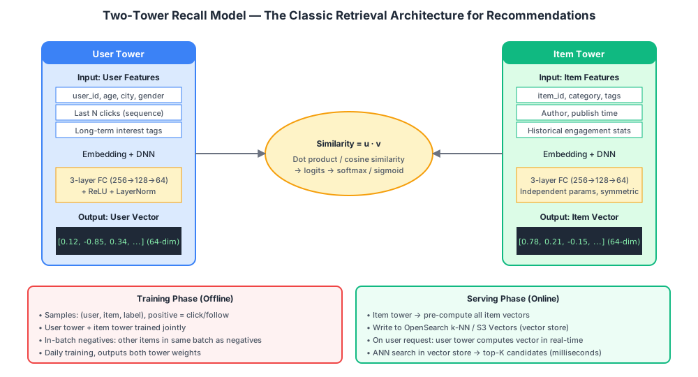
Model Architecture#

Two independent neural networks (“towers”):

• User tower: Consumes user features → outputs a 64-dim or 128-dim vector
• Item tower: Consumes item features → outputs a vector of the same dimensionality
• The dot product or cosine similarity of the two = the user’s preference score for the item

score(user, item) = user_embedding · item_embedding

Training#

Samples = (user, item, label), where positive samples are actual clicks or follows.

Key technique — in-batch negatives: Other users’ positive samples within the same batch serve as negative samples for the current user (no need to explicitly sample negatives).

Loss functions: softmax cross-entropy / sampled softmax / BPR loss.

Serving (The Key Insight)#

Why the two-tower model is easy to deploy — because the user tower and item tower are decoupled, enabling offline precomputation:

After training:
  1. Use the item tower to precompute vectors for every item on the platform
     (tens of millions of items × 64 dimensions)
  2. Write all vectors into a vector store (OpenSearch k-NN / S3 Vectors)
  3. When a user request arrives, only run the user tower in real-time
     to compute the user vector (< 10ms)
  4. Query the vector store for the K nearest neighbors (millisecond-level ANN search)
  5. Return top-K candidate items

→ This is the essence of how two-tower enables "real-time recall":
  item vectors precomputed + ANN retrieval

ANN: Approximate Nearest Neighbor#

With hundreds of millions of item vectors, exact nearest-neighbor search is too expensive. So we use approximate algorithms:

• HNSW (Hierarchical Navigable Small World) — current mainstream
• IVF + PQ — Faiss family, quantization saves memory
• ScaNN (Google)

Sacrificing minimal precision (recall@100 drops 1–2%), latency goes from seconds to milliseconds.

OpenSearch k-NN supports Faiss / Lucene / nmslib backends: as of 2026, Faiss is the production choice (best performance + quantization + GPU support). Lucene suits small-scale pure-JVM use cases. nmslib is deprecated and should no longer be used.

---

Feature Engineering: 90% of the Work Lives Here#

“Garbage in, garbage out.” — Feature quality determines the model’s upper bound.

Feature Categories#

User-side:

• Static: age, gender, city, registration age
• Short-term behavior: last 5 clicks, dwell time in the past hour (real-time features)
• Long-term preferences: frequently viewed tags, time-of-day patterns, traffic sources
• Social: follower count, following count, friend activity level

Item-side:

• Static: author, category, tags, creation time
• Statistics: impressions, CTR, like rate, completion rate
• Dynamic: trending status, recent comment count

User-Item cross features:

• User’s historical interactions with this author
• User’s preference score for this tag
• Similar content the user recently viewed

Context:

• Time (morning / afternoon / evening), day of week, holidays
• Device, network (WiFi / cellular)
• Geographic location

How Features Are Organized in the Data Warehouse#

ads_user_features        -- User-side (daily batch update)
  user_id, age, city, last_5_click_tags, ...

ads_post_features        -- Item-side (hourly update)
  post_id, category, ctr_7d, like_rate, ...

ads_user_pair_features   -- Cross features (on demand)
  user_id, target_user_id, common_tags, ...

user_realtime_features   -- Real-time (DynamoDB / Flink maintained)
  user_id, last_click_seq[5], session_duration, ...

Feature Data Flow#

[ods_event] → [dwd_user_action] → [dws_user_daily] → [ads_user_features]  ← daily batch
                                                          │
                                                          ▼
                                                  Sync to DynamoDB
                                                          │
                                                          ▼
                                                  Real-time point lookup at inference

[MSK events] → Flink real-time compute last 5 clicks → DynamoDB user_realtime_features
                                                          │
                                                          ▼
                                                  Real-time point lookup at inference

---

PIT Correctness (The Most Common Pitfall)#

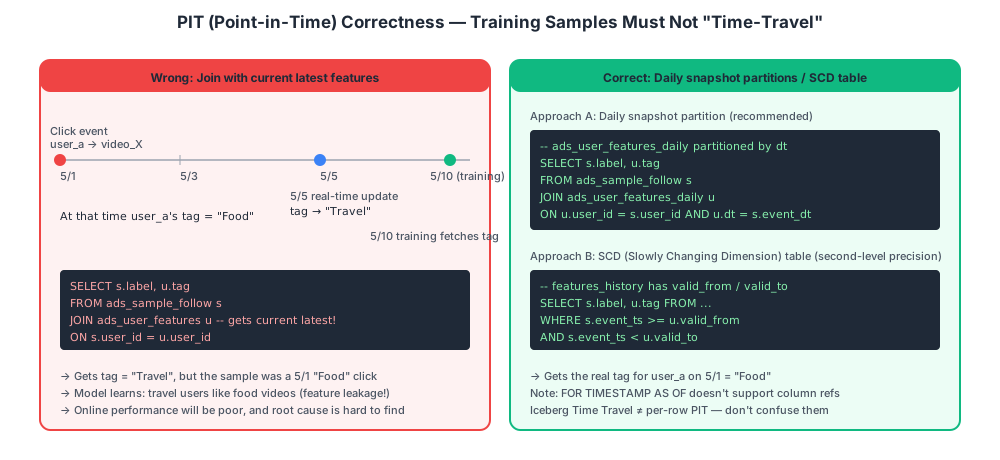
The Problem#

Training samples must use feature values as they existed at the moment the event occurred, not the latest current values.

Otherwise → feature leakage: the model uses “future” information, offline AUC looks great, but online performance is terrible.

Example#

• On May 1, User A clicks Video X (a positive sample)
• On May 1, A’s interest tag = “food”
• On May 5, A browses videos and the algorithm updates the tag to “travel”
• On May 10, during training, a naive JOIN ads_user_features ON user_id = A → retrieves “travel”
• The model learns: “travel” users click food videos → wrong

Solutions#

Warning: Correcting a widespread misconception: Many articles suggest JOIN ads_user_features FOR TIMESTAMP AS OF s.event_ts — this is incorrect. In Iceberg / SQL:2011, FOR TIMESTAMP AS OF only accepts literal constants, not column references. See Part 2 of this series for details.

Solution A: Daily Feature Snapshot Partitions (Recommended, Most Common)

-- ads_user_features_daily partitioned by dt, with a full snapshot written daily
SELECT s.label, u.tag, u.age
FROM   ads_sample_follow s
JOIN   ads_user_features_daily u
       ON u.user_id = s.user_id
       AND u.dt    = s.event_dt;   -- Join on the day's snapshot

Precision: day-level. Use Iceberg expire_snapshots to control storage costs.

Solution B: Slowly Changing Dimension (SCD Type 2, second-level precision)

user_id  tag    valid_from           valid_to
A        food   2026-04-01 00:00     2026-05-05 12:00
A        travel 2026-05-05 12:00     2999-12-31 23:59

SELECT s.label, u.tag
FROM   ads_sample_follow s
JOIN   ads_user_features_history u
       ON s.user_id = u.user_id
       AND s.event_ts >= u.valid_from
       AND s.event_ts <  u.valid_to;

Precision: second-level. More storage-efficient (only adds rows on changes).

Solution C: SageMaker Feature Store

A managed PIT feature store; call get_record(record_id, event_time) and it automatically returns the value as of that moment. Under the hood, it wraps Solution A/B. See Ch09 for details.

Iceberg Time Travel: Real Value Beyond PIT#

Although it cannot do per-row PIT joins, Time Travel remains critical for:

• Data rollback: Recover from accidental deletes or updates
• Reproducible training: Pin a snapshot ID to produce identical samples months later
• Auditing / debugging: Compare “yesterday’s table at midnight” with “today’s table at midnight”

→ The complete solution for recommendation scenarios is Iceberg + daily snapshot partitions + SCD tables. Time Travel is an auxiliary capability.

Why This Is the Critical Lifeline#

New ML engineers building training samples almost always make this mistake. Offline AUC of 0.85 looks beautiful, but online CTR doesn’t budge — the root cause is feature leakage. This is the “classic pitfall” of recommendation engineering. Choose from Solution A/B/C — do not go down the non-existent path of per-row Time Travel.

---

Real-Time Features: What Flink Does#

Some features are short-lived and high-frequency, requiring real-time maintenance:

Real-Time Feature	Description
Last 5 clicks	Behavior sequence for DIN-style models
Dwell time in the last hour	Interest intensity signal
Current session action sequence	Short-term intent modeling
Current network / device / time slot	Context

Implementation:

MSK events
   │
   ▼
Flink Job (keyBy user_id)
   │
   ├─ Sliding Window (5 min)
   ├─ State: maintain each user's last N clicks list (RocksDB)
   │
   ▼
DynamoDB user_realtime_features
   user_id → { last_5_clicks: [...], session_dur: 300, ... }
   │
   ▼
Recommendation inference service point lookup (milliseconds)

Latency: from user click → visible in DynamoDB, single-digit seconds.

---

Model Type Overview#

Recall Models#

Model	Use Case
Collaborative Filtering (CF)	Classic; works as long as you have an interaction matrix
Two-Tower	Mainstream; essential for social scenarios
Graph Neural Network (GNN)	Effective when relationship data is rich (social networks)
Sequential Models (SASRec / BERT4Rec)	Behavior sequence modeling

Ranking Models#

Model	Use Case
LightGBM / XGBoost	Simple and reliable; strong feature engineering can beat many deep models
DeepFM	DNN + FM; balances feature crossing and depth
Wide & Deep	Google’s classic architecture
DIN (Deep Interest Network)	Alibaba; attention over behavior sequences
Transformer	Heavy; excellent results but expensive
MMoE / PLE	Multi-task (optimize click + completion + follow simultaneously)

Practical Recommendations for Customer Scenarios#

POC phase (within 6 months):

• Recall: Collaborative Filtering + Two-Tower (OpenSearch k-NN)
• Pre-ranking: Can be omitted
• Ranking: LightGBM (first) → DeepFM
• Re-ranking: Business rules (diversity, spread)

Advanced phase:

• GNN recall (Neptune ML)
• DIN / SIM ranking (behavior sequence modeling)
• Multi-channel recall fusion (learned weights)

---

Offline Evaluation Metrics#

Metric	Stage	Meaning
Recall@K	Recall	Does top-K retrieval hit the actual clicks?
Hit Rate	Recall	Similar to Recall
AUC	Ranking	Discrimination ability (0.5 = random, 1.0 = perfect)
NDCG@K	Ranking	Weighted ranking quality
GAUC	Ranking	AUC computed per-user then weighted (closer to online performance)

Warning: High offline AUC does not equal good online performance. Common causes: PIT errors, data leakage, ignoring exposure bias. A/B testing is the ground truth.

---

A/B Testing#

Deploying a model does not mean rolling it out to all users immediately. You must A/B test:

All users
  ├─ 50% (Control group A) → Old model
  └─ 50% (Experiment group B) → New model

Observe for N days, compare core business metrics:
  - CTR (Click-Through Rate)
  - User dwell time
  - Retention rate
  - GMV / Business conversion

If the new model is significantly better (statistically p < 0.05 and business metrics improve) → full rollout.

A/B testing platforms are often built in-house (GrowthBook / Optimizely / custom); this guide does not expand on that topic.

---

Chapter Summary#

Concept	One-Liner
Recommendation Funnel	Candidate pool → Recall → Pre-Rank → Rank → Re-Rank
Recall	Don’t miss; hundreds of millions → thousands; multi-channel parallel
Ranking	Rank accurately; thousands → tens; heavy models
Two-Tower	Mainstream recall model; item tower precomputed + ANN retrieval
Feature Engineering	User / item / cross / context; 90% of the work
PIT	Use feature values from the moment of the event; leverage Iceberg Time Travel
Real-Time Features	Flink maintains short-term high-frequency features; writes to DynamoDB